Spark Applications

Spark Applications consist of a driver process and a set of executor processes.

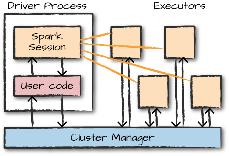
The driver process runs your main() function, sits on a node in the cluster, and is responsible for three things:

• maintaining information about the Spark Application;
• responding to a user’s program or input;
• and analyzing, distributing, and scheduling work across the executors (discussed momentarily).

The driver process is absolutely essential—it’s the heart of a Spark Application and maintains all relevant information during the lifetime of the application.

The executors are responsible for actually carrying out the work that the driver assigns them. This means that each executor is responsible for only two things:

• executing code assigned to it by the driver;
• and reporting the state of the computation on that executor back to the driver node.

SparkSession

SparkContext & HiveContext & SqlContext

In previous versions of Spark, the SQLContext and HiveContext provided the ability to work with DataFrames and Spark SQL and were commonly stored as the variable sqlContext in examples, documentation, and legacy code. As a historical point, Spark 1.X had effectively two contexts. The SparkContext and the SQLContext. These two each performed different things. The former focused on more fine-grained control of Spark’s central abstractions, whereas the latter focused on the higher-level tools like Spark SQL. In Spark 2.X, the communtiy combined the two APIs into the centralized SparkSession that we have today. However, both of these APIs still exist and you can access them via the SparkSession. It is important to note that you should never need to use the SQLContext and rarely need to use the SparkContext.

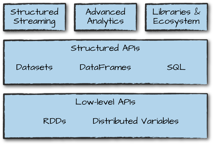
Structured API

The majority of the Structured APIs apply to both batch and streaming computation. This means that when you work with the Structured APIs, it should be simple to migrate from batch to streaming (or vice versa) with little to no effort.

DataFrame

All “DataFrame”s are actually Datasets of type Row.

A DataFrame is the most common Structured API and simply represents a table of data with rows and columns. The list that defines the columns and the types within those columns is called the schema. You can think of a DataFrame as a spreadsheet with named columns. A spreadsheet sits on one computer in one specific location, whereas a Spark DataFrame can span thousands of computers. The reason for putting the data on more than one computer should be intuitive: either the data is too large to fit on one machine or it would simply take too long to perform that computation on one machine.

type DataFrame = Dataset[Row]

Schemas

A schema defines the column names and types of a DataFrame. You can define schemas manually or read a schema from a data source (often called schema on read). Schemas consist of types, meaning that you need a way of specifying what lies where.

Dataset: Type-Safe Structured APIs

The first API we’ll describe is a type-safe version of Spark’s structured API called Datasets, for writing statically typed code in Java and Scala.

The “untyped” DataFrames and the “typed” Datasets. To say that DataFrames are untyped is aslightly inaccurate; they have types, but Spark maintains them completely and only checks whether those types line up to those specified in the schema at runtime. Datasets, on the other hand, check whether types conform to the specification at compile time. Datasets are only available to Java Virtual Machine (JVM)–based languages (Scala and Java) and we specify types with case classes or Java beans.

When you’re using DataFrames, you’re taking advantage of Spark’s optimized internal format. To Spark (in Scala), DataFrames are simply Datasets of Type Row. The “Row” type is Spark’s internal representation of its optimized in-memory format for computation. This format makes for highly specialized and efficient computation because rather than using JVM types, which can cause high garbage-collection and object instantiation costs, Spark can operate on its own internal format without incurring any of those costs.

DataFrames and Datasets are (distributed) table-like collections with well-defined rows and columns. Each column must have the same number of rows as all the other columns (although you can use null to specify the absence of a value) and each column has type information that must be consistent for every row in the collection. To Spark, DataFrames and Datasets represent immutable, lazily evaluated plans that specify what operations to apply to data residing at a location to generate some output. When we perform an action on a DataFrame, we instruct Spark to perform the actual transformations and return the result. These represent plans of how to manipulate rows and columns to compute the user’s desired result.

SQL tables and views

Tables and views are basically the same thing as DataFrames. We just execute SQL against them instead of DataFrame code.

Overview of Structured API Execution

This section will demonstrate how this code is actually executed across a cluster. This will help you understand (and potentially debug) the process of writing and executing code on clusters, so let’s walk through the execution of a single structured API query from user code to executed code. Here’s an overview of the steps:

1. Write DataFrame/Dataset/SQL Code.
2. If valid code, Spark converts this to a Logical Plan.
3. Spark transforms this Logical Plan to a Physical Plan, checking for optimizations along the way.
4. Spark then executes this Physical Plan (RDD manipulations) on the cluster.

Basic Structured Operations

Columns as expressions

(((col("someCol") + 5) * 200) - 6) < col("otherCol")

import org.apache.spark.sql.functions.expr
expr("(((someCol + 5) * 200) - 6) < otherCol")

Repartition and Coalesce

Repartition will incur a full shuffle of the data.

Coalesce will not incur a full shuffle and will try to combine partitions. This operation will shuffle your data into five partitions based on the destination country name, and then coalesce them (without a full shuffle):

df.repartition(5, col("DEST_COUNTRY_NAME")).coalesce(2)

To see more, check “ch05”.

RDD(Resilient Distributed Datasets)

RDDs being a lower-level representation of Datasets. DataFrame operations are built on top of RDDs and compile down to these lower-level tools for convenient and extremely efficient distributed execution.

Virtually everything in Spark is built on top of RDDs.

Partitions

To allow every executor to perform work in parallel, Spark breaks up the data into chunks called partitions. A partition is a collection of rows that sit on one physical machine in your cluster. A DataFrame’s partitions represent how the data is physically distributed across the cluster of machines during execution. If you have one partition, Spark will have a parallelism of only one, even if you have thousands of executors. If you have many partitions but only one executor, Spark will still have a parallelism of only one because there is only one computation resource.

An important thing to note is that with DataFrames you do not (for the most part) manipulate partitions manually or individually. You simply specify high-level transformations of data in the physical partitions, and Spark determines how this work will actually execute on the cluster. Lower-level APIs do exist (via the RDD interface).

Spark has several core abstractions: Datasets, DataFrames, SQL Tables, and Resilient Distributed Datasets (RDDs). These different abstractions all represent distributed collections of data. The easiest and most efficient are DataFrames, which are available in all languages.

Transformations

In Spark, the core data structures are immutable, meaning they cannot be changed after they’re created.

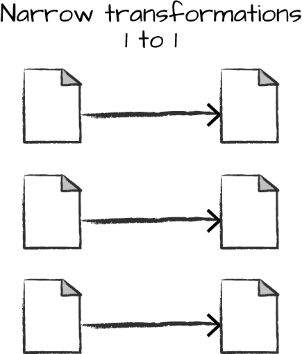
narrow dependencies(narrow transformations)

Only one partition contributes to at most one output partition.(like operation filter)

wide dependency(wide transformations)

Input partitions contributing to many output partitions.(like operation shuffle)

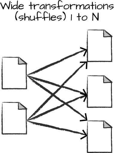
With narrow transformations, Spark will automatically perform an operation called pipelining, meaning that if we specify multiple filters on DataFrames, they’ll all be performed in-memory. The same cannot be said for shuffles. When we perform a shuffle, Spark writes the results to disk.

Lazy Evaluation

Logical Plan VS Physical Plan

 flightData2015.sort("count").explain()

== Physical Plan ==
*Sort [count#195 ASC NULLS FIRST], true, 0
+- Exchange rangepartitioning(count#195 ASC NULLS FIRST, 200)
   +- *FileScan csv [DEST_COUNTRY_NAME#193,ORIGIN_COUNTRY_NAME#194,count#195] ...

DataFrames and SQL

You can express your business logic in SQL or DataFrames (either in R, Python, Scala, or Java) and Spark will compile that logic down to an underlying plan(that you can see in the explain plan) before actually executing your code. With Spark SQL, you can register any DataFrame as a table or view (a temporary table) and query it using pure SQL. There is no performance difference between writing SQL queries or writing DataFrame code, they both “compile” to the same underlying plan that we specify in DataFrame code.

 flightData2015.createOrReplaceTempView("flight_data_2015")

val sqlWay = spark.sql("""
SELECT DEST_COUNTRY_NAME, count(1)
FROM flight_data_2015
GROUP BY DEST_COUNTRY_NAME
""")

val dataFrameWay = flightData2015
  .groupBy('DEST_COUNTRY_NAME)
  .count()

sqlWay.explain
dataFrameWay.explain

== Physical Plan ==
*HashAggregate(keys=[DEST_COUNTRY_NAME#182], functions=[count(1)])
+- Exchange hashpartitioning(DEST_COUNTRY_NAME#182, 5)
   +- *HashAggregate(keys=[DEST_COUNTRY_NAME#182], functions=[partial_count(1)])
      +- *FileScan csv [DEST_COUNTRY_NAME#182] ...
== Physical Plan ==
*HashAggregate(keys=[DEST_COUNTRY_NAME#182], functions=[count(1)])
+- Exchange hashpartitioning(DEST_COUNTRY_NAME#182, 5)
   +- *HashAggregate(keys=[DEST_COUNTRY_NAME#182], functions=[partial_count(1)])
      +- *FileScan csv [DEST_COUNTRY_NAME#182] ...

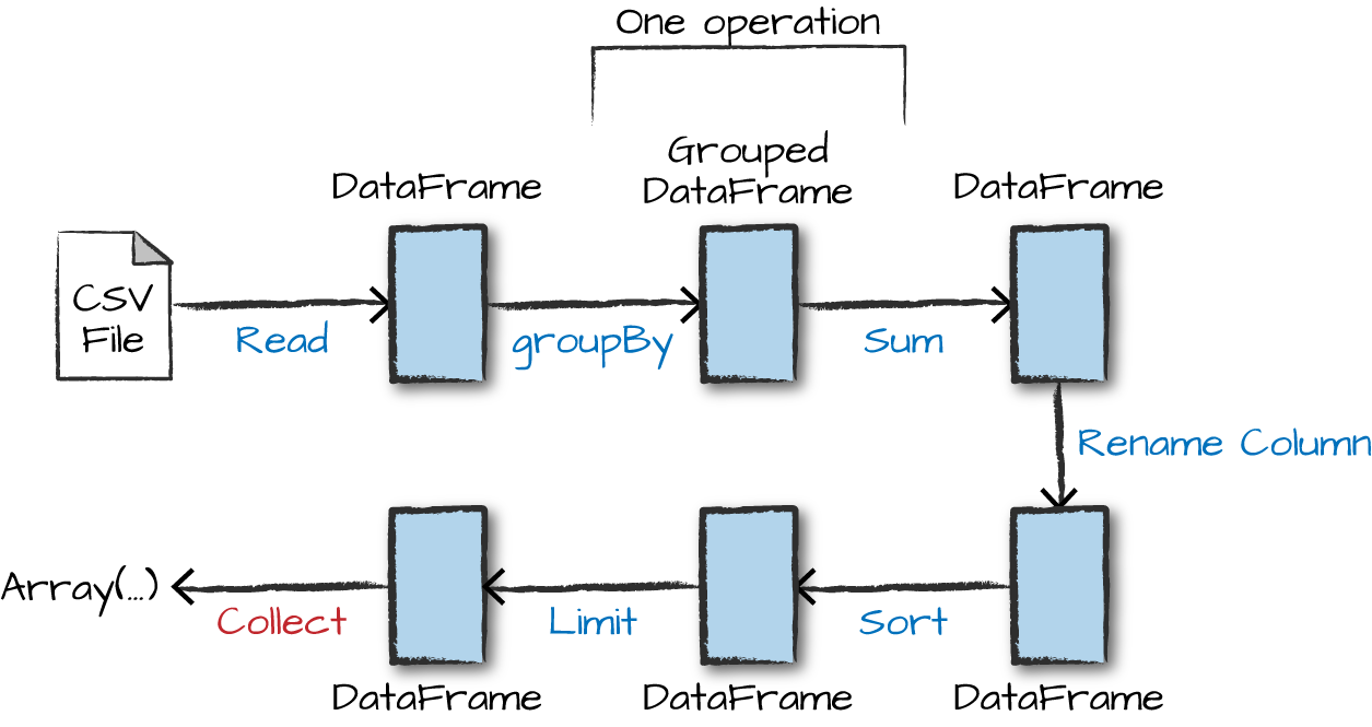
import org.apache.spark.sql.functions.desc

flightData2015
  .groupBy("DEST_COUNTRY_NAME")
  .sum("count")
  .withColumnRenamed("sum(count)", "destination_total")
  .sort(desc("destination_total"))
  .limit(5)
  .show()

This execution plan is a directed acyclic graph (DAG) of transformations, each resulting in a new immutable DataFrame, on which we call an action to generate a result.

Stream Processing

Structured Streaming

With Structured Streaming, you can take the same operations that you perform in batch mode using Spark’s structured APIs and run them in a streaming fashion. This can reduce latency and allow for incremental processing. The best thing about Structured Streaming is that it allows you to rapidly and quickly extract value out of streaming systems with virtually no code changes. It also makes it easy to conceptualize because you can write your batch job as a way to prototype it and then you can convert it to a streaming job. The way all of this works is by incrementally processing that data.

The DStream API

The DStreams API has several limitations. First, it is based purely on Java/Python objects and functions, as opposed to the richer concept of structured tables in DataFrames and Datasets. This limits the engine’s opportunity to perform optimizations. Second, the API is purely based on processing time to handle event-time operations, applications need to implement them on their own. Finally, DStreams can only operate in a micro-batch fashion, and exposes the duration of micro-batches in some parts of its API, making it difficult to support alternative execution modes.

Structured Streaming

Structured Streaming has native support for event time data (all of its the windowing operators automatically support it). As of Apache Spark 2.2, the system only runs in a micro-batch model, but the Spark team at Databricks has announced an effort called Continuous Processing to add a continuous execution mode. This should become an option for users in Spark 2.3.

batch job:

spark.read...

stream job:

spark.readStream...

...writeStream...

Original link：https://pages.databricks.com/definitive-guide-spark.html